Introduction

This article explains how to compute and visualize a simple scalar function f(x) = x^2 + 20 and its derivative grad(x) = 2x using Python. You will learn why the derivative is zero at an extremum, how a decreasing sequence of x values affects the gradient, and how to plot both the function and its gradient with NumPy and Matplotlib. The content is practical, reproducible, and optimized for search and answer engines.

Why this example matters

The quadratic function f(x) = x^2 + 20 is a canonical example in calculus and optimization. It has a single global minimum at x = 0. At that extremum point the derivative is zero, which is the core concept used in optimization algorithms such as gradient descent. When you generate a sequence of decreasing positive x values, the gradient (which is 2x) also decreases in magnitude toward zero.

Quick Python example

Here is a compact script that demonstrates generating a decaying sequence of x values, computing f(x) and grad(x), then printing a numeric example:

 # sequence and simple function/gradient
s = [10.0]
for _ in range(5):
    s.append(s[-1] * 0.98)

loss = lambda x: (x**2) + 20
grad = lambda x: x * 2

w = 9.8
print(loss(w), grad(w))

This prints the function value and gradient at w = 9.8. As w decreases toward 0, grad(w) decreases linearly because grad(w) = 2w.

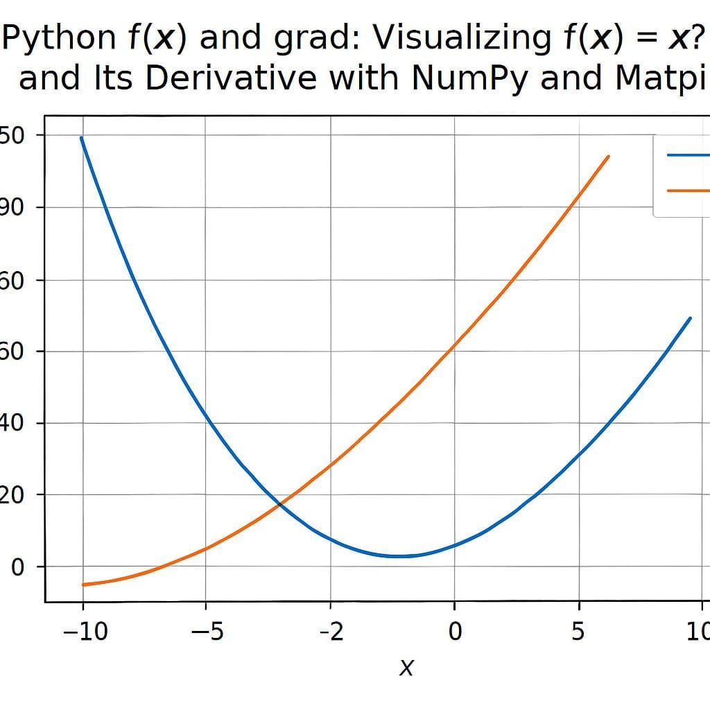
Plotting f(x) and grad(x) with NumPy and Matplotlib

To visualize the relationship between the function and its derivative, generate a longer decaying sequence and plot both values. The following code creates 100 points that decay by multiplying by 0.98 each step, computes f(x) and grad(x), and plots them in different colors:

import matplotlib.pyplot as plt
import numpy as np

w = [10.0]
for _ in range(100):
    w.append(w[-1] * 0.98)

x = np.array(w)
y = np.power(x, 2) + 20
y_grad = x * 2

plt.figure(figsize=(10, 6))
plt.xlim(10, 0)  # reverse x-axis to show decay from left to right
plt.scatter(x, y, label='f(x)', color='blue')
plt.scatter(x, y_grad, label='grad(x)', color='red')
plt.grid()
plt.legend()
plt.tight_layout()
plt.show()

Note the use of plt.xlim(10, 0) which flips the x-axis so that the decay appears left to right. The blue points are the values of f(x); the red points are the gradient values. As x approaches 0, the red points move toward 0, illustrating the derivative becoming zero at the minimum.

Key observations

Extremum and derivative: For f(x) = x^2 + 20 the minimum is at x = 0 and the derivative equals zero there.
Gradient behavior: When x is positive and decreasing, grad(x) = 2x also decreases toward 0. The gradient sign indicates the slope direction: positive for x > 0, negative for x < 0.
Visualization: Plotting both f(x) and grad(x) side by side helps build intuition about how the slope changes across x values.

Practical tips and alternatives

Use NumPy arrays instead of Python lists for faster numeric operations when working with many points: x = np.array(s).
To generate sequences without loops, consider vectorized approaches: x = 10.0 * (0.98 ** np.arange(N)).
Functional styles such as map or list comprehensions can be used for small transformations: list(map(lambda v: v*2, lst)) or [v*2 for v in lst].
To demonstrate optimization, you can show a simple gradient descent update: w = w – lr * grad(w) with a small learning rate lr.

Common questions

What does derivative zero mean? It means the instantaneous slope is zero and the point is a local extremum for differentiable functions.
Why use x^2 + 20? The constant 20 shifts the function upward without changing location of the minimum, making it a clean example for visualization.
How to extend to 2D? For f(x, y) you can compute gradients as partial derivatives and visualize as a contour or heatmap to show level sets and gradient fields.

Conclusion

This example is a simple, effective way to connect calculus concepts to practical Python visualization. By computing f(x) = x^2 + 20 and grad(x) = 2x over a decaying sequence, you can clearly see how the gradient approaches zero at the extremum. Use NumPy for efficient arrays and Matplotlib for clear plots. These building blocks are directly relevant to optimization and machine learning workflows.

Python f(x) and grad: Visualizing f(x)=x^2+20 and Its Derivative with NumPy and Matplotlib